Step 3: fit_p

YuKi

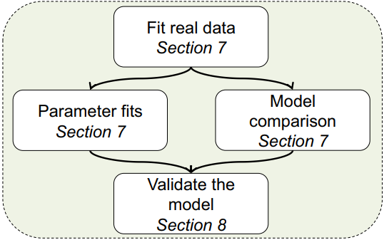
Estimate Methods

With minimal configuration, users can estimate optimal parameters using four distinct methods. In the following code snippets, I only highlight the arguments that vary by estimation method. Unless explicitly noted, other arguments can be duplicated from the above example.

# How to use MLE as estimate method
fitting.MLE <- multiRL::fit_p(
  estimate = "MLE",
  control = list(
    core = 10, sample = 100, iter = 100
  ),
  ...
)
# How to use MAP as estimate method
fitting.MAP <- multiRL::fit_p(
  estimate = "MAP",
  control = list(
    core = 10, sample = 100, iter = 100,
    diff = 0.001, patience = 10
  ),
  ...
)
# How to use ABC as estimate method
fitting.ABC <- multiRL::fit_p(
  estimate = "ABC",
  control = list(
    core = 10, sample = 100, train = 1000,
    tol = 0.1
  ),
  ...
)

# How to use RNN as estimate method
reticulate::use_condaenv(condaenv = "your_tensorflow_env_name", required = TRUE)

fitting.RNN <- multiRL::fit_p(
  estimate = "RNN",
  control = list(
    core = 1, sample = 100, train = 1000,
    layer = "GRU", units = 128, batch_size = 10, epochs = 100
  ),
  ...
)

Note
All of the following figures were generated using multiRL::rpl_e()

Demo

MLE

fitting.MLE <- multiRL::fit_p(
  estimate = "MLE",

  data = data,
  behrule = behrule,
  colnames = colnames,

  models = list(multiRL::TD, multiRL::RSTD, multiRL::Utility),
  settings = list(name = c("TD", "RSTD", "Utility")),
  
  algorithm = "NLOPT_GN_MLSL",
  lowers = list(c(0, 0), c(0, 0, 0), c(0, 0, 0)),
  uppers = list(c(1, 10), c(1, 1, 10), c(1, 10, 1)),
  control = list(core = 10, iter = 100)
)

save(fitting.MLE, file = "./fitting.MLE.Rdata")

MAP

fitting.MAP <- multiRL::fit_p(
  estimate = "MAP",

  data = data,
  behrule = behrule,
  colnames = colnames,

  models = list(multiRL::TD, multiRL::RSTD, multiRL::Utility),
  priors = list(
    list(
      alpha = function(x) {stats::dbeta(x, shape1 = 2, shape2 = 2, log = TRUE)}, 
      beta = function(x) {stats::dexp(x, rate = 1, log = TRUE)}
    ),
    list(
      alphaN = function(x) {stats::dbeta(x, shape1 = 2, shape2 = 2, log = TRUE)}, 
      alphaP = function(x) {stats::dbeta(x, shape1 = 2, shape2 = 2, log = TRUE)}, 
      beta = function(x) {stats::dexp(x, rate = 1, log = TRUE)}
    ),
    list(
      alpha = function(x) {stats::dbeta(x, shape1 = 2, shape2 = 2, log = TRUE)}, 
      beta = function(x) {stats::dexp(x, rate = 1, log = TRUE)},
      gamma = function(x) {stats::dbeta(x, shape1 = 2, shape2 = 2, log = TRUE)}
    )
  ),
  settings = list(name = c("TD", "RSTD", "Utility")),
  
  algorithm = "NLOPT_GN_MLSL",
  lowers = list(c(0, 0), c(0, 0, 0), c(0, 0, 0)),
  uppers = list(c(1, 10), c(1, 1, 10), c(1, 10, 1)),
  control = list(
    core = 10, iter = 100,
    diff = 0.1, patience = 1
  )
)

save(fitting.MAP, file = "./fitting.MAP.Rdata")

ABC

fitting.ABC <- multiRL::fit_p(
  estimate = "ABC",

  data = data,
  behrule = behrule,
  colnames = colnames,

  models = list(multiRL::TD, multiRL::RSTD, multiRL::Utility),
  priors = list(
    list(
      alpha = function(x) {stats::rbeta(n = 1, shape1 = 2, shape2 = 2)}, 
      beta = function(x) {stats::rexp(n = 1, rate = 1)}
    ),
    list(
      alphaN = function(x) {stats::rbeta(n = 1, shape1 = 2, shape2 = 2)}, 
      alphaP = function(x) {stats::rbeta(n = 1, shape1 = 2, shape2 = 2)}, 
      beta = function(x) {stats::rexp(n = 1, rate = 1)}
    ),
    list(
      alpha = function(x) {stats::rbeta(n = 1, shape1 = 2, shape2 = 2)}, 
      beta = function(x) {stats::rexp(n = 1, rate = 1)},
      gamma = function(x) {stats::rbeta(n = 1, shape1 = 2, shape2 = 2)}
    )
  ),
  settings = list(name = c("TD", "RSTD", "Utility")),
  
  lowers = list(c(0, 0), c(0, 0, 0), c(0, 0, 0)),
  uppers = list(c(1, 10), c(1, 1, 10), c(1, 10, 1)),
  control = list(
    core = 10, train = 1000,
    tol = 0.1
  )
)

save(fitting.ABC, file = "./fitting.ABC.Rdata")

RNN

reticulate::use_condaenv(condaenv = "tf-gpu", required = TRUE)

#> Show in New Window
#> -------------------------------------------------------------------
#> reticulate::use_condaenv(condaenv = "tensorflow", required = TRUE)
#> -------------------------------------------------------------------
#> 
#> Please confirm you have loaded TensorFlow into R (enter 1 or 2). 
#> 
#> 1: Yes, it is loaded
#> 2: No, it is not loaded

fitting.RNN <- multiRL::fit_p(
  estimate = "RNN",

  data = data,
  behrule = behrule,
  colnames = colnames,

  models = list(multiRL::TD, multiRL::RSTD, multiRL::Utility),
  priors = list(
    list(
      alpha = function(x) {stats::rbeta(n = 1, shape1 = 2, shape2 = 2)}, 
      beta = function(x) {stats::rexp(n = 1, rate = 1)}
    ),
    list(
      alphaN = function(x) {stats::rbeta(n = 1, shape1 = 2, shape2 = 2)}, 
      alphaP = function(x) {stats::rbeta(n = 1, shape1 = 2, shape2 = 2)}, 
      beta = function(x) {stats::rexp(n = 1, rate = 1)}
    ),
    list(
      alpha = function(x) {stats::rbeta(n = 1, shape1 = 2, shape2 = 2)}, 
      beta = function(x) {stats::rexp(n = 1, rate = 1)},
      gamma = function(x) {stats::rbeta(n = 1, shape1 = 2, shape2 = 2)}
    )
  ),
  settings = list(name = c("TD", "RSTD", "Utility")),
  
  lowers = list(c(0, 0), c(0, 0, 0), c(0, 0, 0)),
  uppers = list(c(1, 10), c(1, 1, 10), c(1, 10, 1)),
  control = list(
    core = 1, train = 1000,
    layer = "GRU", units = 128, batch_size = 10, epochs = 100
  )
)

save(fitting.RNN, file = "./fitting.RNN.Rdata")

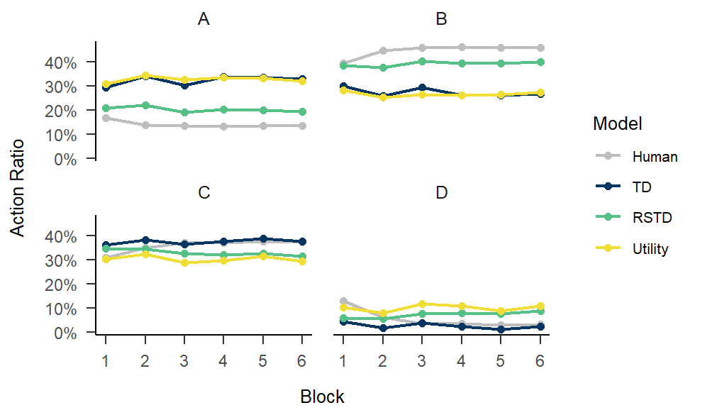
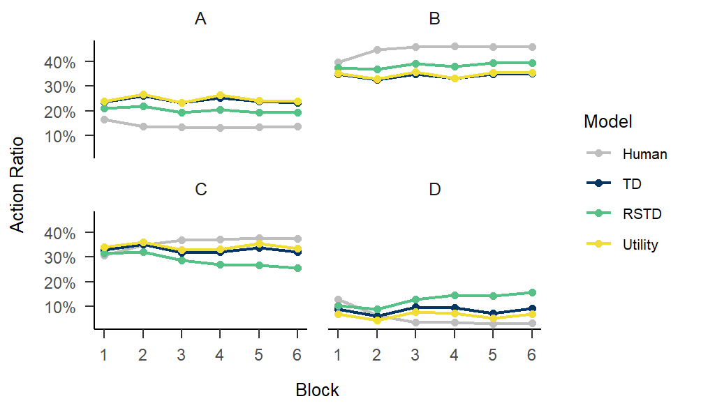
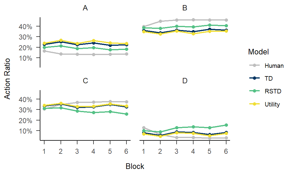
Comparison

Despite employing identical computational models with synchronized hyper-parameter settings (e.g., a fixed lapse rate of 0.1), the resulting parameter estimates exhibit substantial discrepancies across different estimation methods. Remarkably, all four estimation techniques had previously demonstrated robust parameter recovery capabilities in simulated environments.

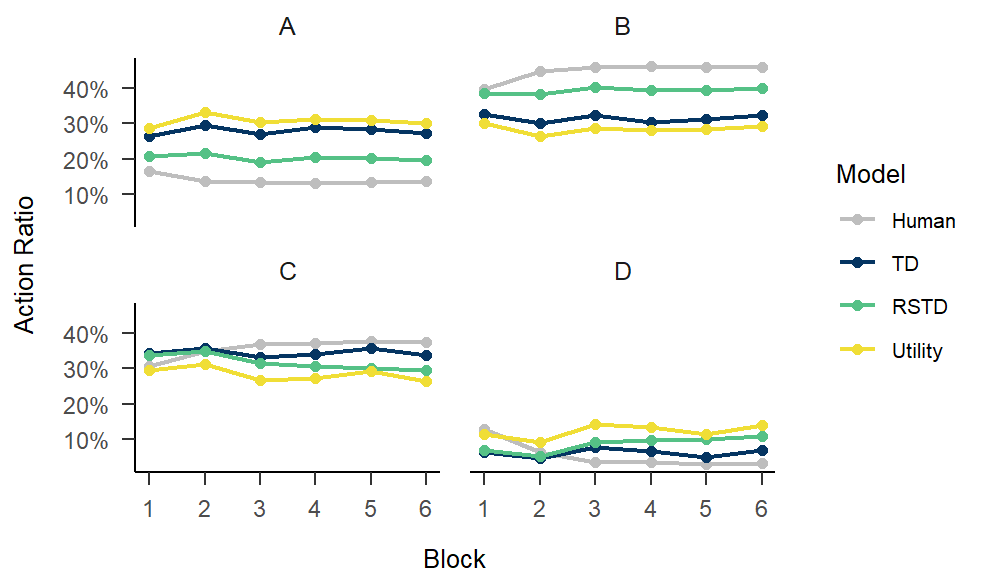
As illustrated in the figure below, the probability density functions (PDFs) of the “optimal” parameters vary significantly by method. For instance, MLE and MAP tend to yield estimates clustered around extreme boundaries (near 0 or 1).

Furthermore, when examining the pairwise correlations between the optimal parameters, the convergence remains strikingly low. Only the MLE and MAP estimates for \(\alpha\) show a moderate-to-high correlation, whereas almost no meaningful associations exist between other pairs of estimation techniques.