Recurrent Neural Networks

YuKi

Traditional methods like MLE, MAP, MCMC all operate on a similar principle: they start with a set of parameters, run a reinforcement learning model to generate a sequence of choices, and then evaluate the similarity between this simulated sequence and the human subject’s behavior to determine if the parameters are optimal.

In contrast, Recurrent Neural Network (RNN) uses a reverse approach. It takes a large number of choice sequences, each generated by different parameters, as input, and parameters that generated those sequences, as output. By training this large-scale model, a direct mapping between behavior and parameters is established. Once the neural network is trained, it can be given a new sequence of choices and can directly infer which parameters likely generated it.

Install Packages

# You need to accept three terms of the conda license to install Miniconda.
conda tos accept --override-channels --channel https://repo.anaconda.com/pkgs/main
conda tos accept --override-channels --channel https://repo.anaconda.com/pkgs/r
conda tos accept --override-channels --channel https://repo.anaconda.com/pkgs/msys2

reticulate::install_miniconda()

Install TensorFlow according to system and CPU/GPU

# To run TensorFlow, you need to downgrade NumPy.
conda install numpy=1.26.4

Simulating Data

list_simulated <- binaryRL::simulate_list(
  data = binaryRL::Mason_2024_G2,
  id = 1,
  obj_func = binaryRL::TD,
  n_params = 2,
  n_trials = 360,
  lower = c(0, 0),
  upper = c(1, 1),
  iteration = 1100 # = [800(train) + 200(test)] + [100(recovery)]
)

n_sample = 1000
n_trials = 360
n_info = 3
n_params = 2

Step 1: List to Matrix

# create NULL list
X_list<- list()
Y_list <- list()

# obtain options
unique_L <- unique(list_simulated[[1]]$data$L_choice)
unique_R <- unique(list_simulated[[1]]$data$R_choice)
options <- sort(unique(c(unique_L, unique_R)))
options <- as.vector(options)

# as.matrix
for (i in 1:n_sample) {
  
  # Input Info: L_choice, R_choice, Sub_Choose
  X_list[[i]] <- as.matrix(
    data.frame(
      L_choice = match(
        x = list_simulated[[i]]$data$L_choice, 
        table = options
      ),
      R_choice = match(
        x = list_simulated[[i]]$data$R_choice, 
        table = options
      ),
      Choose = match(
        x = list_simulated[[i]]$data$Sub_Choose, 
        table = options
      )
    )
  )
  
  # Output Info: RL Model Parameters
  Y_list[[i]] <- as.matrix(
    do.call(
      what = data.frame,
      args = lapply(
        X = 1:length(list_simulated[[i]]$input),
        FUN = function(j) {
          list_simulated[[i]]$input[[j]]
        }
      )
    )
  )
}

Step 2: Matrix to Array

# Input: n_sample, n_trials, n_info
X <- array(NA, dim = c(n_sample, n_trials, n_info))

for (i in 1:n_sample) {
  X[i, , ] <- X_list[[i]]
}

# Output: n_sample, n_params
Y <- array(NA, dim = c(n_sample, n_params))

for (i in 1:n_sample) {
  Y[i, ] <- Y_list[[i]]
}

Step 3: Train & Test

X_train <- X[1:(n_sample*0.8), , , drop = FALSE]
Y_train <- Y[1:(n_sample*0.8), , drop = FALSE]

X_test <- X[(n_sample*0.8+1):n_sample, , , drop = FALSE]
Y_test <- Y[(n_sample*0.8+1):n_sample, , drop = FALSE]

Step 4: Training RNN Model

#reticulate::use_condaenv("tf-cpu", required = TRUE)
reticulate::use_condaenv("tf-gpu", required = TRUE)

# Initialize Model (sequential decision making)
Model <- keras::keras_model_sequential()

algorithm = "GRU"
#algorithm = "LSTM"

# Recurrent Layer
switch(
  EXPR = algorithm, 
  "GRU" = {
    Model <- keras::layer_gru(
      object = Model,
      units = 128,
      input_shape = c(n_trials, n_info), 
      return_sequences = FALSE, 
    ) 
  },
  "LSTM" = {
    Model <- keras::layer_lstm(
      object = Model,
      units = 128,
      input_shape = c(n_trials, n_info), 
      return_sequences = FALSE, 
    ) 
  },
) |>
  # Hidden Layer
  keras::layer_dense(
    units = 64, 
    activation = "relu"
  ) |>
  # Output Layer
  keras::layer_dense(
    units = n_params, 
    activation = "linear"
  ) |>
  # Loss Function
  keras::compile(
    loss = "mean_squared_error",
    optimizer = "adam",
    metrics = c("mean_absolute_error")
  )

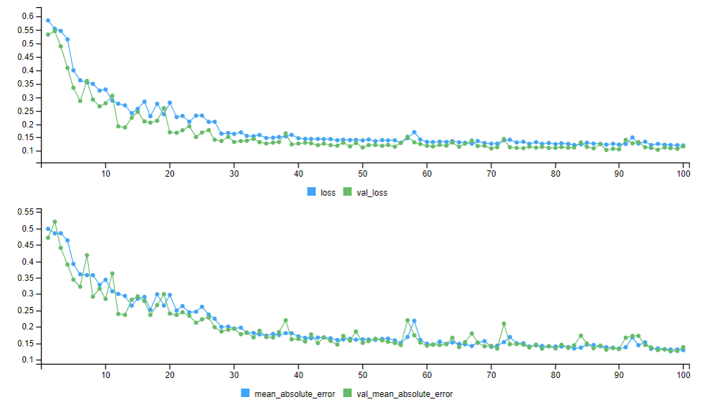
# Training RNN Model
history <- Model |>
  keras::fit(
  x = X_train,
  y = Y_train,
  epochs = 100,
  batch_size = 10,
  validation_data = list(X_test, Y_test),
  verbose = 2
)

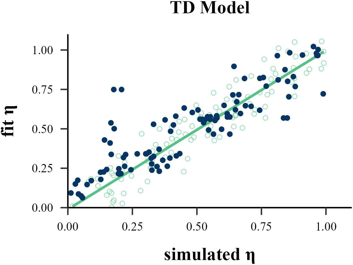
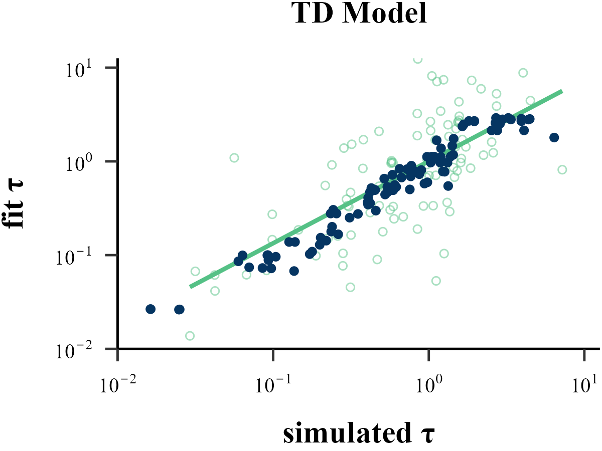
Parameter Recovery

X_pred_list <- vector("list", length = 100) 
X_true_list <- vector("list", length = 100)

for (i in (n_sample + 1):(n_sample + 100)) {

  X_sub <- array(NA, dim = c(1, n_trials, n_info))
  
  X_sub[1, , ] <- as.matrix(
    data.frame(
      L_choice = match(
        x = list_simulated[[i]]$data$L_choice, 
        table = options
      ),
      R_choice = match(
        x = list_simulated[[i]]$data$R_choice, 
        table = options
      ),
      Choose = match(
        x = list_simulated[[i]]$data$Sub_Choose, 
        table = options
      )
    )
  )

################################## [core] ######################################
  X_pred <- predict(object = Model, x = X_sub)
################################## [core] ######################################
  
  X_pred_list[[i - n_sample]] <- X_pred
  X_true_list[[i - n_sample]] <- list_simulated[[i]]$input
}

df_true <- as.data.frame(do.call(rbind, X_true_list))
df_pred <- as.data.frame(do.call(rbind, X_pred_list))

cor(df_true$V1, df_pred$V1)
cor(df_true$V2, df_pred$V2)

[1] 0.8988817
[1] 0.8428525

rm(unique_L, unique_R)
rm(X_list, Y_list)
rm(X, Y)
rm(algorithm, X_train, X_test, Y_train, Y_test)
rm(i, X_sub, X_pred, n_sample, n_trials, n_info, n_params, options)
rm(X_pred_list, X_true_list)