Traditional methods like MLE, MAP, MCMC all operate on a similar principle: they start with a set of parameters, run a reinforcement learning model to generate a sequence of choices, and then evaluate the similarity between this simulated sequence and the human subject’s behavior to determine if the parameters are optimal.
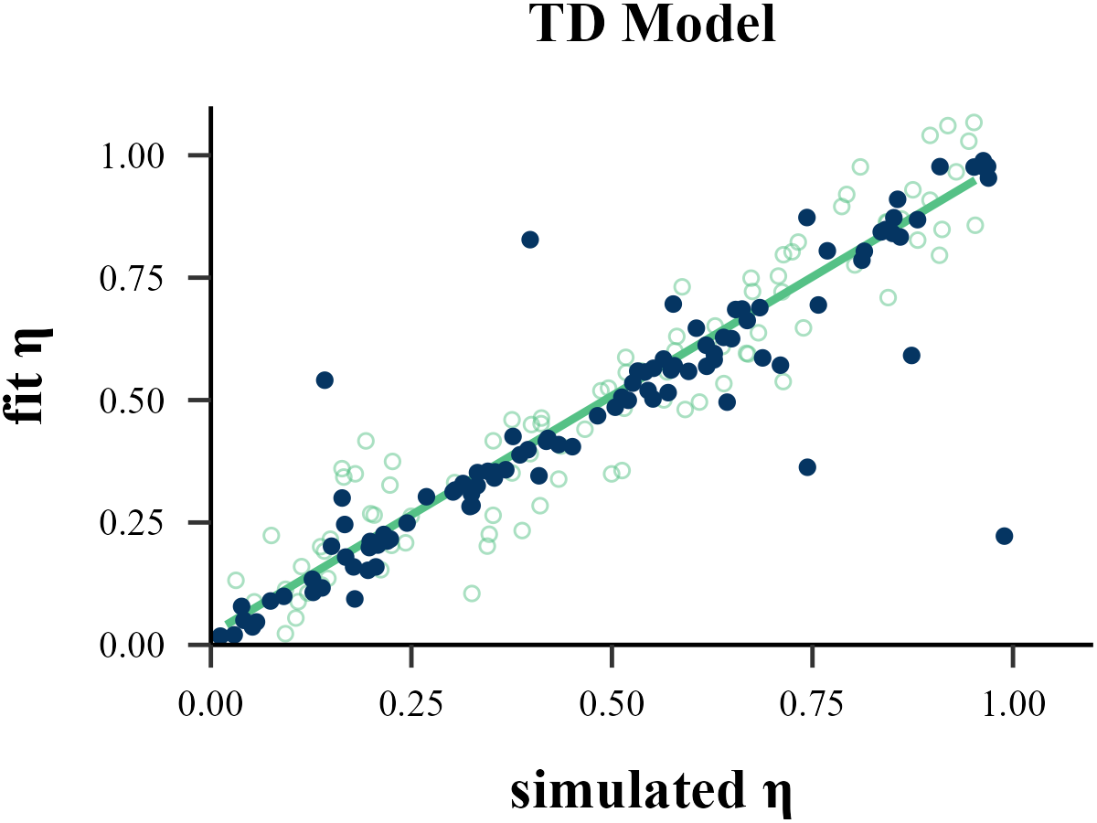
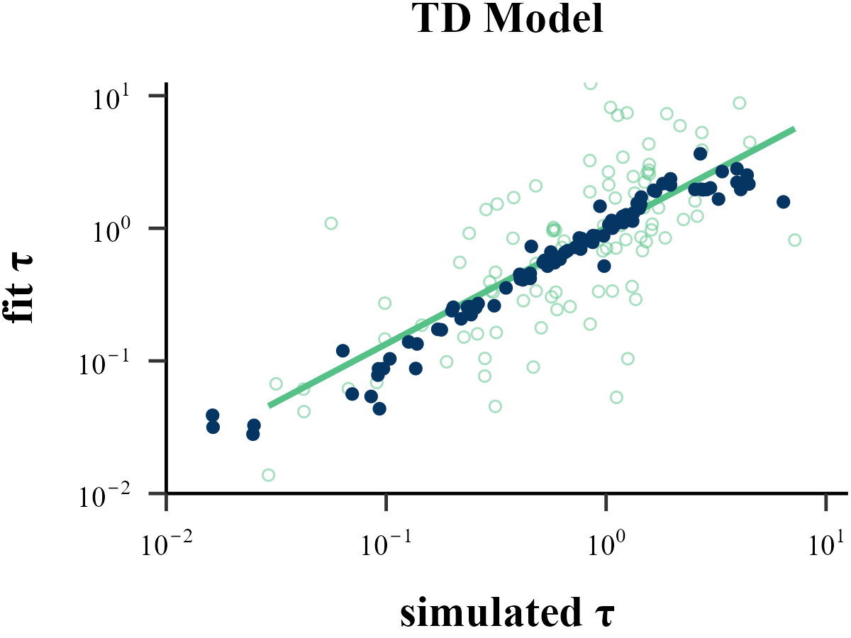
Approximate Bayesian Computation (ABC) follows a similar Recurrent Neural Network (RNN). However, instead of learning a direct mapping from the entire behavioral sequence to the parameters, ABC focuses on the relationship between the input parameters and a set of summary statistics derived from the output. By condensing the full behavioral data into these key statistical features, ABC requires significantly less information and computational resources than a sequence-based model like an RNN. Crucially, despite this simplification, ABC often yields parameter recovery results that are substantially more robust and accurate than those from traditional methods like MLE.
Install Package
install.packages("abc")Simulating Data
list_simulated <- binaryRL::simulate_list(
  data = binaryRL::Mason_2024_G2,
  id = 1,
  n_params = 2,
  n_trials = 360,

  obj_func = binaryRL::TD,
  rfun = list(
    eta = function() { stats::runif(n = 1, min = 0, max = 1) },
    tau = function() { stats::rexp(n = 1, rate = 1) }
  ),
  iteration = 1100 # = [1000(train) + 100(valid)]]
)

list_train <- list_simulated[1:1000]
list_valid <- list_simulated[1001:1100]
Step 1: Free Parameters
extract_params <- function(x) {
  param_vector <- x$input
  names(param_vector) <- c("eta", "tau")
  return(param_vector)
}

# parameters for training
df_train.params <- dplyr::bind_rows(
  .x = purrr::map(.x = list_train, .f = extract_params)
)

df_valid.params <- dplyr::bind_rows(
  .x = purrr::map(.x = list_valid, .f = extract_params)
)
Step 2: Summary Statistics
extract_sumstats <- function(x) {
  x[["data"]] %>%
    dplyr::filter(Frame %in% c("Gain", "Loss")) %>%
    dplyr::mutate(
      Risky = case_when(
        Sub_Choose %in% c("A", "C") ~ 0,
        Sub_Choose %in% c("B", "D") ~ 1
      )
    ) %>%
    dplyr::group_by(Block) %>%
    dplyr::summarise(
      mean_risky = mean(Risky),
      sd_risky = sd(Risky),
    ) %>%
    tidyr::pivot_longer(
      cols = -Block,
      names_to = "metric",
      values_to = "value"
    ) %>%
    tidyr::pivot_wider(
      names_from = c(Block, metric),
      values_from = value
    )
}

# summary statistics for training
df_train.sumstats <- dplyr::bind_rows(
  .x = purrr::map(.x = list_train, .f = extract_sumstats)
)

# summary statistics for validation
df_valid.sumstats <- dplyr::bind_rows(
  .x = purrr::map(.x = list_valid, .f = extract_sumstats)
)
Step 3: Training ABC Model
df_true <- df_valid.params
df_pred <- data.frame(
  eta = NA,
  tau = NA
)

for (i in 1:100) {
  result <- abc::abc(
    target = as.vector(df_valid.sumstats[i, ]),
    param = df_train.params,
    sumstat = df_train.sumstats,
    tol = .1,
    method = "neuralnet",
    transf = c("logit", "none"),
    logit.bounds = rbind(c(0, 1), c(NA, NA))
  )

  df_pred[i, ] <- summary(result)[5, ]
}